Cantor expansions of integers

My answer is based on a Cantor expansion of the integers. The binary representation of integer numbers is well-known. In R, use this function to get it:

number2binary <- function(number, noBits=1+floor(log2(max(number,1)))) {
  if(noBits < 1+floor(log2(number))) warning(sprintf("noBits=%s is not enough", noBits))
  return( as.numeric(intToBits(number))[1:noBits] ) 
}
number2binary(5)
## [1] 1 0 1
number2binary(5, noBits=4)
## [1] 1 0 1 0

The second argument, noBits, allows to fix the length of the binary representation, adding some 0 to the right to reach it.

The binary representation is a system of numerotation. The correspondence between the usual decimal representation and the binary representation is the following:

nmax <- 10
data.frame(
  N=0:nmax,
  expansion=vapply(0:nmax, function(i) paste(myutils::number2binary(i), collapse=""), character(1))
)
##     N expansion
## 1   0         0
## 2   1         1
## 3   2        10
## 4   3        11
## 5   4       100
## 6   5       101
## 7   6       110
## 8   7       111
## 9   8      1000
## 10  9      1001
## 11 10      1010

The numerotation for the \(2^n\) first integers is also given by the Cartesian product of the set \(\{0,1\}\) with itself \(n\) times:

expand.grid(epsilon0=c(0,1), epsilon1=c(0,1), epsilon2=c(0,1))
##   epsilon0 epsilon1 epsilon2
## 1        0        0        0
## 2        1        0        0
## 3        0        1        0
## 4        1        1        0
## 5        0        0        1
## 6        1        0        1
## 7        0        1        1
## 8        1        1        1

Thus, one can view the binary representation of a number \(n\) as the \(n\)-th element of this Cartesian product (for the colexicographic order). The enumeration is easily viewed on a tree:

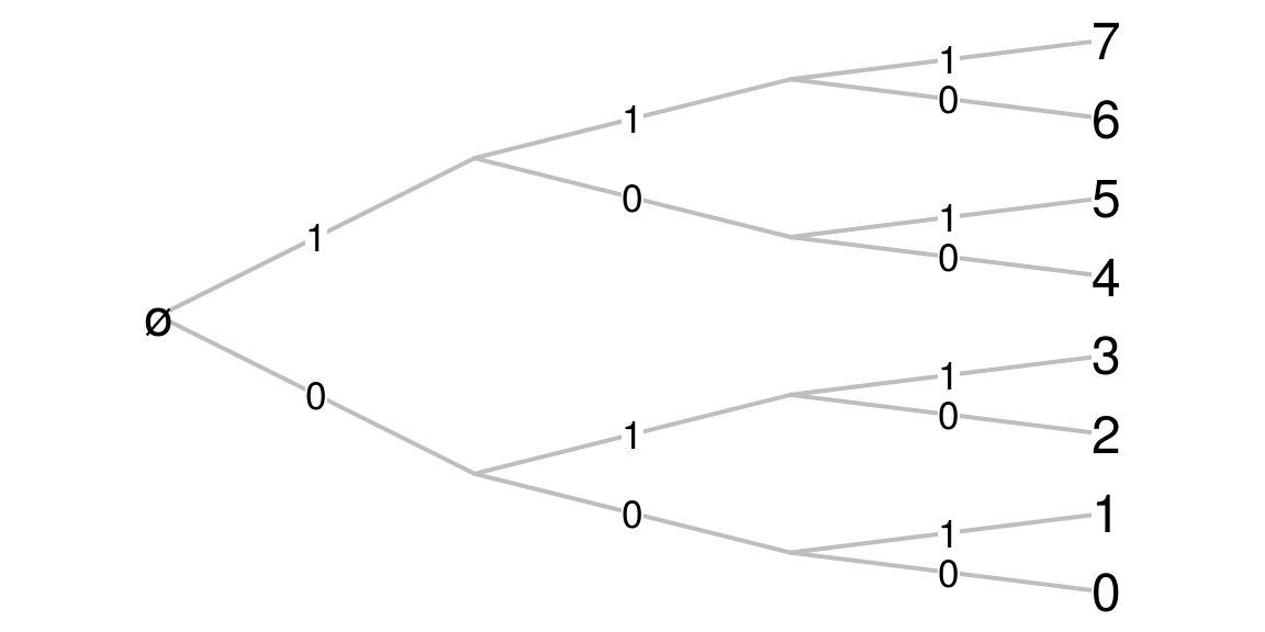
Well, everybody knows that. In mathematical terms, the binary representation allows to write any natural number \(N\) as a finite sequence of digits \(\epsilon_i \in \{0,1\}\): \[ N = \text{"}\epsilon_0\epsilon_1\epsilon_2\ldots\epsilon_n\text{"}. \] and that means \[ N = \epsilon_0 + \epsilon_1\times 2 + \epsilon_2 \times 2^2 + \ldots + \epsilon_n \times 2^n. \]

Such a representation is more generally possible with digits \(\epsilon_i \in \{0,\ldots, r_n-1\}\), where \((r_n)\) is a sequence of integer numbers \(\geq 2\), and then the representation means \[ N = \epsilon_0 + \epsilon_1\times \ell_1 + \epsilon_2 \times \ell_2 + \ldots + \epsilon_n \times \ell_n, \] where \(\ell_n=\prod_{i=0}^{n-1} r_i\), and then this expansion of \(N\) is called its \((r_n)\)-ary expansion. The binary expansion is the case when \(r_n\equiv 2\). The general \((r_n)\)-ary expansion is called a Cantor’s number system. There also are, beyond the scope of this post, more general systems of numeration.

For example, the \((3,4,5)\)-ary representation of a number \(n\) is the \(n\)-th element of this Cartesian product \(\{0,1,2\}\times\{0,1,2,3\}\times\{0,1,2,3,4\}\).

One gets the integer \(N\) from its \((r_n)\)-ary expansion by simply applying the above formula. Conversely, the derivation of the \((r_n)\)-ary from an integer is given by the greedy algorithm:

• While \(N>0\)
  • Take the first index \(k\) such that \(\ell_k > N\)
  • Set \(\epsilon_k\) to be the Euclidean quotient of \(N\) by \(\ell_{k-1}\), and update \(N\) to be the remainder

This R function returns the \((r_n)\)-ary expansion, using the binary expansion as the default one:

intToAry <- function(n, sizes=rep(2, 1+floor(log2(max(n,1))))){
  l <- c(1, cumprod(sizes))
  epsilon <- numeric(length(sizes))
  while(n>0){
    k <- which.min(l<=n)
    e <- floor(n/l[k-1])
    epsilon[k-1] <- e
    n <- n-e*l[k-1]
  }
  return(epsilon)
}
aryToInt <- function(epsilon, sizes=rep(2, length(epsilon)-1)){
  sum(epsilon*c(1,cumprod(sizes[1:(length(epsilon)-1)])))
}

As an example:

intToAry(29, c(3, 4, 5)) 
## [1] 2 1 2

means that \(29 = 2\times 1 + 1 \times 3 + 2 \times (3\times 4)\).

Note that the last element of sizes, here 5, is not visible in the expansion. It only fixes the maximal value of \(\epsilon_2\): the \((3,4,5)\)-ary expansion of \(N\) is \[ N = \epsilon_0 + \epsilon_1 \times 3 + \epsilon_2 \times (3\times 4) \] with \(\epsilon_0 \in \{0,1,2\}\), \(\epsilon_1 \in \{0, 1, 2, 3\}\), \(\epsilon_2 \in \{0, 1, 2, 3, 4\}\).

Application to nested loops

Assume you have a nested loop:

for(i in 1:3){
  for(j in 1:4){
    for(k in 1:5){
      doSomething(c(i,j,k))
    }
  }
}

This nested loop can be reduced to only one loop with the \((3,4,5)\)-ary representation:

for(n in 1:(3*4*5)){
  doSomething(intToAry(n, c(3,4,5)) + 1)
}

A Rcpp implementation

Using the intToAry function in a long loop could be time-consuming. We give below a C++ implementation for R, using the Rcpp and inline packages.

library(inline)
src <- 'int n = as<int>(N);
std::vector<int> s = as< std::vector<int> >(sizes);
std::vector<int> epsilon (s.size());
std::vector<int>::iterator it;
it = s.begin();
it = s.insert ( it , 1 );
int G[s.size()];
std::partial_sum (s.begin(), s.end(), G, std::multiplies<int>());
int k;
while(n>0){
  k=1;
  while(G[k]<=n){
    k=k+1;
  }
  epsilon[k-1] = (int)n / G[k-1];
  n = n % G[k-1];
}
return wrap(epsilon); '
intToAry_Rcpp <- cxxfunction(signature(N="integer",
                           sizes="integer"),
                 body=src, plugin="Rcpp")

intToAry_Rcpp(29, c(3,4,5))
## [1] 2 1 2

L <- vector(mode="list", length=2*3*4*5*6*7*8*9)
system.time(
  for(n in 1:(2*3*4*5*6*7*8*9)){
    L[[n]] <- intToAry(n-1, c(2,3,4,5,6,7,8,9))
  }
)
##    user  system elapsed 
##  14.429   0.000  14.431
system.time(
  for(n in 1:(2*3*4*5*6*7*8*9)){
    L[[n]] <- intToAry_Rcpp(n-1, c(2,3,4,5,6,7,8,9))
  }
)
##    user  system elapsed 
##   1.521   0.000   1.530

A Javascript implementation

function intToAry(n, sizes) {
  if (n<0) throw new Error("n must be a nonnegative integer");
  for (i = 0; i<sizes.length; i++) if (sizes[i]!=parseInt(sizes[i]) || sizes[i]<1){  throw new Error("sizes must be a vector of integers be >1"); };
  for (var G = [1], i = 0; i<sizes.length; i++) G[i+1] = G[i] * sizes[i]; 
  if (n>=_.last(G)) throw new Error("n must be <" + _.last(G));
  for (var epsilon=[], i=0; i < sizes.length; i++) epsilon[i]=0;
  while(n > 0){
    var k = _.findIndex(G, function(x){ return n < x; }) - 1;
    var e = (n/G[k])>>0;
    epsilon[k] = e;
    n = n-e*G[k];
  }
  return epsilon;
}
intToAry(29, [3, 4, 5])
## 2,1,2