The Kantorovich distance between two probability measures $\mu$ and $\nu$ on a finite set $A$ equipped with a metric $d$ is defined as

$$d'(\mu,\nu)= \min_{\Lambda \in {\cal J}(\mu, \nu)} \int d(x,y)\textrm{d}\Lambda(x,y)$$ where ${\cal J}(\mu, \nu)$ is the set of all joinings of $\mu$ and $\nu$, that is, the set of all probability measures $\Lambda$ on $A \times A$ whose margins are $\mu$ and $\nu$.

The Kantorovich distance can also be defined for more general metric spaces $(A,d)$ but our purpose is to show how to compute the Kantorovich distance in R when $A$ is finite.

Actually the main part of the work will be to get the extreme points of the set of joinings ${\cal J}(\mu, \nu)$. Indeed, this set has a convex structure and the numerical application

$${\cal J}(\mu, \nu) \ni \Lambda \mapsto \int d(x,y)\textrm{d}\Lambda(x,y)$$ is linear. Therefore, any extremal value of this application, in particular the Kantorovich distance $d'(\mu,\nu)$, is attained by an extreme joining $\Lambda \in {\cal J}(\mu, \nu)$. This latter point will be explained below, and we will also see that ${\cal J}(\mu, \nu)$ is a convex polyhedron.

Computing extreme joinings in R

What is an extreme joining in ${\cal J}(\mu, \nu)$ ? First of all, what is a joining in ${\cal J}(\mu, \nu)$ ? Consider for instance $A=\{a_1,a_2,a_3\}$ then a joining of $\mu$ and $\nu$ is given by a matrix

$$P=\begin{pmatrix} p_{11} & p_{12} & p_{13} \\ p_{21} & p_{22} & p_{23} \\ p_{31} & p_{32} & p_{33} \end{pmatrix}$$ whose $(i,j)$-th entry $p_{ij}$ is the probability $p_{ij}=\Pr(X=i,Y=j)$ where $X \sim \mu$ and $Y \sim \nu$ are random variables on $A$. Given a distance $d$ on $A$, the Kantorovich distance $d'(\mu,\nu)$ is then the minimal possible value of the mean distance $\mathbb{E}[d(X,Y)]$ between $X$ and $Y$. Note that $\mathbb{E}[d(X,Y)]=\Pr(X \neq Y)$ when taking $d$ as the discrete $0-1$ distance on $A$.

The $H$-representation of ${\cal J}(\mu, \nu)$

The possible values of the $p_{ij}$ satisfy the following three sets of linear equality/inequality constraints:

$$\begin{cases} {\rm (1a) } \quad \sum_j p_{ij} = \mu(a_i) & \forall i \\ {\rm (1b) } \quad \sum_i p_{ij} = \nu(a_j) & \forall j \\ {\rm (2) } \quad p_{ij} \geq 0 & \forall i,j \\ \end{cases}.$$ Considering $P$ written in stacked form : $$P={\begin{pmatrix} p_{11} & p_{12} & p_{13} & p_{21} & p_{22} & p_{23} & p_{31} & p_{32} & p_{33} \end{pmatrix}}'$$ then the first set ${\rm (1a)}$ of linear equality constraints is $M_1 P = \begin{pmatrix} \mu(a_1) \\ \mu(a_2) \\ \mu(a_3) \end{pmatrix}$ with $$M_1 = \begin{pmatrix} 1 & 1 & 1 & 0 & 0 & 0 & 0 & 0 & 0 \\ 0 & 0 & 0 & 1 & 1 & 1 & 0 & 0 & 0 \\ 0 & 0 & 0 & 0 & 0 & 0 & 1 & 1 & 1 \end{pmatrix}$$ and the second set ${\rm (1b)}$ of linear equality constraints is $M_2 P = \begin{pmatrix} \nu(a_1) \\ \nu(a_2) \\ \nu(a_3) \end{pmatrix}$ with $$M_2 = \begin{pmatrix} 1 & 0 & 0 & 1 & 0 & 0 & 1 & 0 & 0 \\ 0 & 1 & 0 & 0 & 1 & 0 & 0 & 1 & 0 \\ 0 & 0 & 1 & 0 & 0 & 1 & 0 & 0 & 1 \end{pmatrix}.$$

With the terminology of the cddlibb library, ${\cal J}(\mu, \nu)$ is a convex polyhedron and the linear constraints above define its H-representation. Schematically, one can imagine ${\cal J}(\mu, \nu)$ as a convex polyhedra embedded in a higher dimensional space:

Your browser does not support the HTML5 canvas element.

Here ${\cal J}(\mu, \nu)$ is a $4$-dimensional convex polyhedron embedded in a $9$-dimensional space: its elements are given by $9$ parameters $p_{ij}$ but they are determined by only $4$ of them because of the linear equality constraints ${\rm (1a)}$ and ${\rm (1b)}$.

Vertices of ${\cal J}(\mu, \nu)$ achieve the Kantorovich distance

In the introduction we mentionned that the application

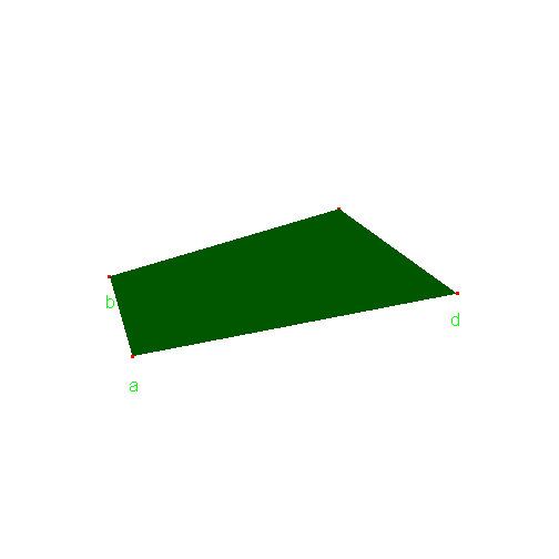
$${\cal J}(\mu, \nu) \ni \Lambda \mapsto \int d(x,y)\textrm{d}\Lambda(x,y)$$ is linear and we claimed that consequently any of its extremal values is attained by an extreme point of ${\cal J}(\mu, \nu)$. Why ?

Extreme points of a convex polyhedron are nothing but its vertices. Consider a point $x$ in a convex polyhedron which is not a vertex, as in the figure below. Then $x$ is a convex combination of the vertices $a$, $b$, $c$, $d$, and therefore the image $\ell(x)$ of $x$ by any linear function $\ell$ is the same convex combination of $\ell(a)$, $\ell(b)$, $\ell(c)$, $\ell(d)$. See figure below, where the polyhedron is in the $xy$-plane and the value of $\ell$ is given on the $z$-axis.

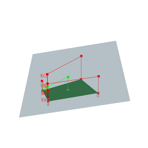
Your browser does not support the HTML5 canvas element.

Consequently, among the four values $\ell(a)$, $\ell(b)$, $\ell(c)$, $\ell(d)$ of $\ell$ at the vertices, there is at least one lower than $\ell(x)$ and at least one higher than $\ell(x)$.

Getting the $V$-representation of ${\cal J}(\mu, \nu)$ and the Kantorovich distance with R

The rccd package for R provides an R interface to the cddlib library. Its main function scdd() performs the conversion between $H$-representation and $V$-representation of a convex polyhedron, which is given by the set of vertices of the convex polyhedron. The set of vertices provide a representation of a polyhedron because each point in the polyhedron is a convex combination of the vertices; we say that the convex polyhedra is the convex hull of its extreme points.

Let us use scdd() to get the vertices of ${\cal J}(\mu, \nu)$. We consider the following example:

mu <- c(1/7,2/7,4/7)
nu <- c(1/4,1/4,1/2)

We firstly define its $H$-representation in a R object with the makeH() function, whose help page begins as follows:

library(rcdd)
help(makeH)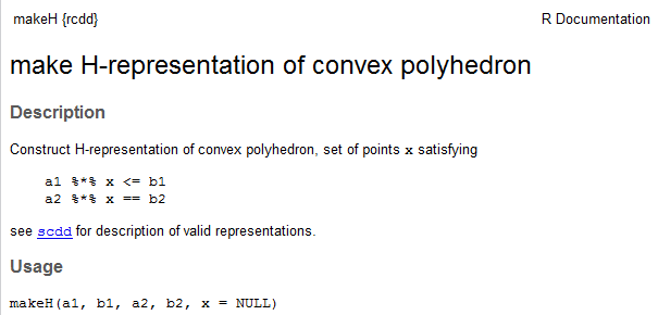

The matrix a1 and the vector b1 specify the linear inequality constraints. Our linear inequality constraints ${\rm 2)}$ are defined in this way in R as follows:

m <- length(mu)
n <- length(nu)
a1 <- -diag(m*n)
b1 <- rep(0,m*n)

The matrix a2 and the vector b2 specify the linear equality constraints. We simply construct b2 by concatenating $\mu$ and $\nu$:

b2 <- c(mu,nu)

The matrix a2 is obtained by stacking the two matrices $M_1$ and $M_2$ defined above. We construct it as follows in R:

M1 <- t(model.matrix(~0+gl(m,n)))[,]
M2 <- t(model.matrix(~0+factor(rep(1:n,m))))[,] 
a2 <- rbind(M1,M2)

Then we can get the vertices of ${\cal J}(\mu, \nu)$ in a list as follows:

H <- makeH(a1,b1,a2,b2)  # H-representation 
V <- scdd(H)$output[,-c(1,2)]  # V-representation (vertices), but not convenient
V <- lapply(1:nrow(V), function(i) matrix(V[i,], ncol=n, byrow=TRUE) )

The command lines below show that there are 15 vertices (extreme joinings) and display the first five of them:

length(V)

## [1] 15

head(V,5)

## [[1]]
##        [,1] [,2]   [,3]
## [1,] 0.1429 0.00 0.0000
## [2,] 0.0000 0.00 0.2857
## [3,] 0.1071 0.25 0.2143
## 
## [[2]]
##        [,1] [,2]   [,3]
## [1,] 0.1429 0.00 0.0000
## [2,] 0.1071 0.00 0.1786
## [3,] 0.0000 0.25 0.3214
## 
## [[3]]
##        [,1]    [,2] [,3]
## [1,] 0.1429 0.00000  0.0
## [2,] 0.1071 0.17857  0.0
## [3,] 0.0000 0.07143  0.5
## 
## [[4]]
##        [,1] [,2]    [,3]
## [1,] 0.1429 0.00 0.00000
## [2,] 0.0000 0.25 0.03571
## [3,] 0.1071 0.00 0.46429
## 
## [[5]]
##         [,1] [,2] [,3]
## [1,] 0.14286 0.00  0.0
## [2,] 0.03571 0.25  0.0
## [3,] 0.07143 0.00  0.5

Now, to get the Kantorovich distance, it suffices to evaluate $\mathbb{E}[d(X,Y)]$ for all extreme joinings, and to take the lower value. Consider for instance the discrete distance $d$. Set it as a matrix in R:

( D <- 1-diag(3) )

##      [,1] [,2] [,3]
## [1,]    0    1    1
## [2,]    1    0    1
## [3,]    1    1    0

sapply(V, function(P){ sum(D*P) })

##  [1] 0.6429 0.5357 0.1786 0.1429 0.1071 0.7857 0.5357 0.4643 0.5714 0.3929
## [11] 0.3929 0.4286 0.9286 0.6071 0.6786

Then call min() to get the Kantorovich distance $d(\mu,\nu)$

Use exact arithmetic !

Are you satisfied ? I'm not: my probability measures $\mu$ and $\nu$ have rational weights, and then the coordinates of the vertices should be rational too.

How to get the vertices in exact rational arithmetic ? Remember my article about the Gauss hypergeometric function. Let's load the gmp package:

library(gmp) 

Actually this is the point suggested by the message appearing when loading rcdd:

library(rcdd)
If you want correct answers, use rational arithmetic.
See the Warnings sections added to help pages for
    functions that do computational geometry.

There's almost nothing to change to our previous code: everything is done in rcdd to handle rational arithmetic. You just have to set the input parameters as bigq numbers. Firstly define $\mu$ and $\nu$ as "bigq" objects:

( mu <- as.bigq(c(1,2,4),7) )

## Big Rational ('bigq') object of length 3:
## [1] 1/7 2/7 4/7

( nu <- as.bigq(c(1,1,1),c(4,4,2)) )

## Big Rational ('bigq') object of length 3:
## [1] 1/4 1/4 1/2

Then define b2 as before:

b2 <- c(mu,nu)

The other input parameters a1, b1, a2 contain integers only, it is more straightforward to convert them. Actually these parameters must be in character mode to input them in the makeH() function, then we convert them as follows:

asab <- function(x) as.character(as.bigq(x))
a1 <- asab(a1)
b1 <- asab(b1)
a2 <- asab(a2)
b2 <- asab(b2)

And now we run exactly the same code as before:

H <- makeH(a1,b1,a2,b2)  # H-representation 
V <- scdd(H)$output[,-c(1,2)]  # V-representation (vertices), but not convenient
V <- lapply(1:nrow(V), function(i) matrix(V[i,], ncol=n, byrow=TRUE) )
head(V,5)

## [[1]]
##      [,1]   [,2]  [,3]  
## [1,] "1/7"  "0"   "0"   
## [2,] "0"    "0"   "2/7" 
## [3,] "3/28" "1/4" "3/14"
## 
## [[2]]
##      [,1]   [,2]  [,3]  
## [1,] "1/7"  "0"   "0"   
## [2,] "3/28" "0"   "5/28"
## [3,] "0"    "1/4" "9/28"
## 
## [[3]]
##      [,1]   [,2]   [,3] 
## [1,] "1/7"  "0"    "0"  
## [2,] "3/28" "5/28" "0"  
## [3,] "0"    "1/14" "1/2"
## 
## [[4]]
##      [,1]   [,2]  [,3]   
## [1,] "1/7"  "0"   "0"    
## [2,] "0"    "1/4" "1/28" 
## [3,] "3/28" "0"   "13/28"
## 
## [[5]]
##      [,1]   [,2]  [,3] 
## [1,] "1/7"  "0"   "0"  
## [2,] "1/28" "1/4" "0"  
## [3,] "1/14" "0"   "1/2"

There's a slight problem when applying the sapply() function to a list of bigq objects. You can use the lapply() function which works well but returns a list:

D <- as.bigq(D)
lapply(V, function(P){ sum(D*P) })

## [[1]]
## Big Rational ('bigq') :
## [1] 9/14
## 
## [[2]]
## Big Rational ('bigq') :
## [1] 15/28
## 
## [[3]]
## Big Rational ('bigq') :
## [1] 5/28
## 
## [[4]]
## Big Rational ('bigq') :
## [1] 1/7
## 
## [[5]]
## Big Rational ('bigq') :
## [1] 3/28
## 
## [[6]]
## Big Rational ('bigq') :
## [1] 11/14
## 
## [[7]]
## Big Rational ('bigq') :
## [1] 15/28
## 
## [[8]]
## Big Rational ('bigq') :
## [1] 13/28
## 
## [[9]]
## Big Rational ('bigq') :
## [1] 4/7
## 
## [[10]]
## Big Rational ('bigq') :
## [1] 11/28
## 
## [[11]]
## Big Rational ('bigq') :
## [1] 11/28
## 
## [[12]]
## Big Rational ('bigq') :
## [1] 3/7
## 
## [[13]]
## Big Rational ('bigq') :
## [1] 13/14
## 
## [[14]]
## Big Rational ('bigq') :
## [1] 17/28
## 
## [[15]]
## Big Rational ('bigq') :
## [1] 19/28

We can't convert this list to a bigq vector with the unlist() function: this does not work, and this is why sapply() does not work too.

To get a vector, use a loop:

distances <- as.bigq(rep(NA,length(V)))
  for(i in 1:length(V)){
        distances[i] <- sum(D*V[[i]])
    }
distances

## Big Rational ('bigq') 15 x 1 matrix:
##       [,1] 
##  [1,] 9/14 
##  [2,] 15/28
##  [3,] 5/28 
##  [4,] 1/7  
##  [5,] 3/28 
##  [6,] 11/14
##  [7,] 15/28
##  [8,] 13/28
##  [9,] 4/7  
## [10,] 11/28
## [11,] 11/28
## [12,] 3/7  
## [13,] 13/14
## [14,] 17/28
## [15,] 19/28

The column structure of distances is unexpected. To get a usual vector, type:

attr(distances,"nrow") <- NULL
distances

## Big Rational ('bigq') object of length 15:
##  [1] 9/14  15/28 5/28  1/7   3/28  11/14 15/28 13/28 4/7   11/28 11/28
## [12] 3/7   13/14 17/28 19/28

The min() function directly works with bigq objects:

( Kantorovich <- min(distances) )

## Big Rational ('bigq') :
## [1] 3/28

To get the numeric evaluation, use:

asNumeric(Kantorovich)

## [1] 0.1071

That's all.