Integer partitions and Young graph

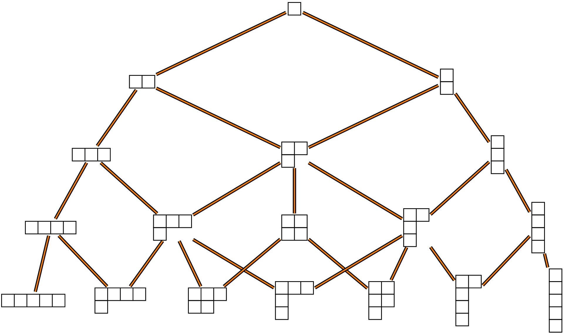
The integer partitions are computed by the parts function of the R package partitions. For example the partitions of \(4\) are obtained as follows:

library(partitions)
parts(4)
##               
## [1,] 4 3 2 2 1
## [2,] 0 1 2 1 1
## [3,] 0 0 0 1 1
## [4,] 0 0 0 0 1

The Young graph is the Bratteli graph whose set of vertices at each level \(n\) is the set of partitions of \(n\) and whose edges connect each partition of weight \(n\) at level \(n\) to its superpartitions of weight \(n+1\) at level \(n+1\).

The R function ymatrices below returns the incidence matrices \(M_n\) of the Young graph.

removezeros <- function(x){ # e.g c(3,1,0,0) -> c(3,1)
  i <- match(0L, x)
  if(!is.na(i)) return(head(x,i-1L)) else return(x)
}
ymatrices <- function(N){
  M <- vector(N, mode="list") 
  M[[1]] <- matrix(1L)
  M[[2]] <- matrix(c(1L,1L), ncol=2)
  M[[3]] <- rbind(c(1L,1L,0L), c(0L,1L,1L))
  colnames(M[[2]]) <- rownames(M[[3]]) <- apply(parts(2), 2, function(x) paste0(removezeros(x), collapse="-"))
  rownames(M[[2]]) <- "1"
  M1 <- parts(3)
  colnames(M[[3]]) <- apply(M1, 2, function(x) paste0(removezeros(x), collapse="-"))
  if(N>3){
    for(k in 4:N){   
      M0 <- M1; M1 <- parts(k)  
      m <- ncol(M0); n <- ncol(M1)
      C <- array(0L, dim=c(m,n))
      rownames(C) <- apply(M0, 2, function(x) paste0(removezeros(x), collapse="-"))
      colnames(C) <- apply(M1, 2, function(x) paste0(removezeros(x), collapse="-"))
      C[1,1:2] <- C[m,c(n-1,n)] <- TRUE
      for(j in 2:(m-1)){
        l <- match(0, M0[,j]) - 1L 
        x <- M0[1L:l,j]
        ss <- c(1L, which(diff(x)<=0)+1L)
        nss <- length(ss)
        connected <- character(nss+1L)
        for(i in seq_len(nss)){
          y <- x
          y[ss[i]] <- y[ss[i]]+1L
          connected[i] <- paste0(y, collapse="-")
        }
        connected[nss+1L] <- paste0(c(x,1L), collapse="-")
        ind <- which(colnames(C) %in% connected)
        C[j,ind] <- 1L
      }
      M[[k]] <- C
    }
  }
  return(M)
}

( Mn <-  ymatrices(4) )
## [[1]]
##      [,1]
## [1,]    1
## 
## [[2]]
##   2 1-1
## 1 1   1
## 
## [[3]]
##     3 2-1 1-1-1
## 2   1   1     0
## 1-1 0   1     1
## 
## [[4]]
##       4 3-1 2-2 2-1-1 1-1-1-1
## 3     1   1   0     0       0
## 2-1   0   1   1     1       0
## 1-1-1 0   0   0     1       1

Standard Young tableaux

A path connecting to the root vertex to a partition \(\lambda\) at level \(n\) corresponds to a standard Young tableau of shape \(\lambda\).

• Number of standard Young tableaux of a given shape. Once we have the incidence matrices of a Bratteli graph, it is easy to compute the number of paths connecting the root vertex to any vertex at a given level. Thus, we get the number of standard Young tableaux of each shape from the incidences matrices \(M_n\). These numbers are returned by the function Flambda below.

Dims <- function(Mn, N){
  Dims <- vector("list", N) 
  Dims[[1]] <- dims0 <- Mn[[1]][1,]
  for(k in 2:N){
    Dims[[k]] <- dims0 <- (dims0 %*% Mn[[k]])[1,] 
  }
  return(Dims)
}
Flambda <- function(N){
  return(Dims(ymatrices(N),N))
}
Flambda(4)
## [[1]]
## [1] 1
## 
## [[2]]
##   2 1-1 
##   1   1 
## 
## [[3]]
##     3   2-1 1-1-1 
##     1     2     1 
## 
## [[4]]
##       4     3-1     2-2   2-1-1 1-1-1-1 
##       1       3       2       3       1

• Paths to a given level. The PathsAtLevel function below returns all the paths of the Young graph going from the partition "1" to the vertices at a given level.

PathsAtLevel <- function(N){
  Mn <- ymatrices(N)[-1]
  f <- function(column, n) sapply(names(which(Mn[[n+1]][column[n],]==1L)), function(x) c(column,x))
  ff <-  function(x, n) lapply(seq_len(ncol(x)), function(i) f(x[, i], n))
  x <- colnames(Mn[[1]])
  if(N > 2) x <- do.call(cbind, sapply(x, f, n=1, simplify=FALSE))
  if(N > 3){
    for(i in 2:(N-2L)){
      x <- do.call(cbind, ff(x,i))
    }
  }
  out <- rbind("1", x)
  rownames(out) <- 1:N
  out <- do.call(cbind, lapply(colnames(Mn[[N-1L]]), function(part) out[, which(colnames(out)==part), drop=FALSE]))
  names(dimnames(out)) <- c("level", "partition")
  return(out)
}
PathsAtLevel(4)
##      partition
## level 4   3-1   3-1   3-1   2-2   2-2   2-1-1   2-1-1   2-1-1   1-1-1-1  
##     1 "1" "1"   "1"   "1"   "1"   "1"   "1"     "1"     "1"     "1"      
##     2 "2" "2"   "2"   "1-1" "2"   "1-1" "2"     "1-1"   "1-1"   "1-1"    
##     3 "3" "3"   "2-1" "2-1" "2-1" "2-1" "2-1"   "2-1"   "1-1-1" "1-1-1"  
##     4 "4" "3-1" "3-1" "3-1" "2-2" "2-2" "2-1-1" "2-1-1" "2-1-1" "1-1-1-1"

• Paths to a given vertex. The PathsToVertex function below returns all the paths of the Young graph going from the partition "1" to a given vertex.

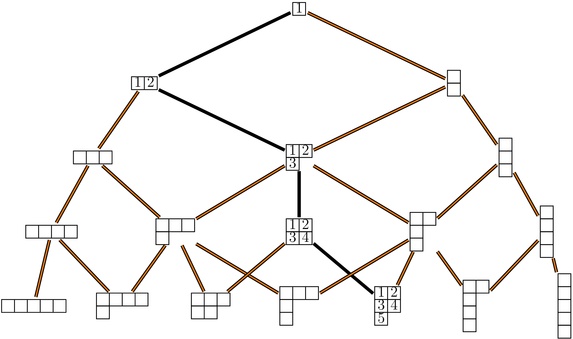
string2letters <- function(string){ # e.g. "abc" -> c("a","b","c")
  rawToChar(charToRaw(string), multiple = TRUE)
}
PathsToVertex <- function(vertex){
  N <- sum(as.integer(string2letters(vertex)[(1:nchar(vertex))%%2L==1L]))
  Mn <- ymatrices(N+1)[-1]
  f <- function(row, n) sapply(names(which(Mn[[n-1]][,row[1]]==1L)), function(x) c(x,row))
  ff <-  function(x, n) lapply(seq_len(ncol(x)), function(i) f(x[, i], n))
  x <- vertex
  x <- f(x, n=N)
  for(i in 1:(N-3L)){
    x <- do.call(cbind, ff(x, N-i))
  }
  x <- rbind("1", x)
  colnames(x) <- NULL
  rownames(x) <- 1:N
  return(x)
}
PathsToVertex("3-2")
##   [,1]  [,2]  [,3]  [,4]  [,5] 
## 1 "1"   "1"   "1"   "1"   "1"  
## 2 "2"   "2"   "1-1" "2"   "1-1"
## 3 "3"   "2-1" "2-1" "2-1" "2-1"
## 4 "3-1" "3-1" "3-1" "2-2" "2-2"
## 5 "3-2" "3-2" "3-2" "3-2" "3-2"

• Convert path to tableau. A path from the partition "1" to a vertex \(\lambda\) corresponds to a standard Young tableau. The path2sy function below returns the standard Young tableau corresponding to a given path.

charpart2vec <- function(x){ # e.g. "3-1-1" -> c(3,1,1,0,0)
  p <- as.integer(string2letters(x)[(1:nchar(x))%%2L==1L])
  out <- rep(0L, sum(p))
  out[seq_along(p)] <- p
  return(out)
}
path2sy <- function(path){
  v <- tail(path,1)
  SY <- rep(list(NULL), (nchar(v)+1)/2) 
  SY[[1]] <- 1L
  for(k in 2:length(path)){
    x <- path[k-1L]; y <- path[k]
    i <- which(charpart2vec(y)-c(charpart2vec(x),0L) == 1L)
    SY[[i]] <- c(SY[[i]], k)
  }
  attr(SY, "path") <- path 
  return(SY)
}
path2sy(c("1", "2", "2-1", "3-1", "3-1-1"))
## [[1]]
## [1] 1 2 4
## 
## [[2]]
## [1] 3
## 
## [[3]]
## [1] 5
## 
## attr(,"path")
## [1] "1"     "2"     "2-1"   "3-1"   "3-1-1"

Plancherel measure and Plancherel growth process

• The Plancherel probability measure \(\mu_n\) on the set of integer partitions of \(n\) is given by \[ \mu_n(\lambda) = \frac{{(f^\lambda)^2}}{n!}, \] where \(f^\lambda\) is the number of standard Young tableaux of shape \(\lambda\). It is returned by the Mu function below. I use the gmp package to get the result in rational numbers.

library(gmp)
Mu <- function(N, mode=c("bigq", "numeric", "character")){
  flambda <- Flambda(N)
  mu <- lapply(1:N, function(i) as.bigq(flambda[[i]]^2, factorialZ(i)))
  if(match.arg(mode)=="numeric"){
    mu <- lapply(mu, as.numeric)
    for(n in 1:N) names(mu[[n]]) <- names(flambda[[n]])
  }
  if(match.arg(mode)=="character"){
    mu <- lapply(mu, as.character)
    for(n in 1:N) names(mu[[n]]) <- names(flambda[[n]])
  }
  return(mu)
}
Mu(4)
## [[1]]
## Big Rational ('bigq') :
## [1] 1
## 
## [[2]]
## Big Rational ('bigq') object of length 2:
## [1] 1/2 1/2
## 
## [[3]]
## Big Rational ('bigq') object of length 3:
## [1] 1/6 2/3 1/6
## 
## [[4]]
## Big Rational ('bigq') object of length 5:
## [1] 1/24 3/8  1/6  3/8  1/24

It is not possible to name the elements a bigq vector. The option mode="numeric" or mode="character" returns the vectors in numeric mode or character mode, with names:

Mu(3, "numeric")
## [[1]]
## [1] 1
## 
## [[2]]
##   2 1-1 
## 0.5 0.5 
## 
## [[3]]
##         3       2-1     1-1-1 
## 0.1666667 0.6666667 0.1666667
Mu(3, "character")
## [[1]]
## [1] "1"
## 
## [[2]]
##     2   1-1 
## "1/2" "1/2" 
## 
## [[3]]
##     3   2-1 1-1-1 
## "1/6" "2/3" "1/6"

• The incidence matrices \(M_n\) easily allow to get the transition probabilities of the Plancherel growth process, using the Vershik-Kerov formula. They are returned by the following function. I use the gmp package to get exact results.

library(gmp)
Plancherel <- function(N, mode=c("bigq", "numeric", "character")){
  Mn <- ymatrices(N+1L)
  Y <- Dims(Mn, N+1L)[-1]
  Mn <- Mn[-1]
  Q <- vector(N, mode="list") 
  Q[[1]] <- t(as.matrix(as.bigq(c(1,1),c(2,2)))) 
  Q[[2]] <- matrix(c(as.bigq(c(1,2,0),3), as.bigq(c(0,2,1),3)), nrow=2, byrow=TRUE) 
  for(k in 3:N){   
    C <- Mn[[k]] 
    m <- nrow(C); n <- ncol(C)
    y <- rep(NA, n); y[n] <- 1L
    Y0 <- Y[[k-1L]]
    Y1 <- Y[[k]]
    q <- as.bigq(matrix(NA, nrow=m, ncol=n))
    for(i in 1:m){
      q[i,] <- C[i,]*as.bigz(Y1)/as.bigz(Y0[i])/(k+1L)
    }
    Q[[k]] <- q
  }
  return(Q)
  if((mode <- match.arg(mode)) != "bigq"){
    convert <- if(mode=="numeric") as.numeric else as.character
    v <- ifelse(mode=="numeric", 0, "")
    for(k in 1:N){
      Qbigq <- Q[[k]]
      Qnum <-  matrix(v, nrow=dim(Qbigq)[1], ncol=dim(Qbigq)[2])
      for(i in 1:nrow(Qnum)){
        Qnum[i,] <- convert(Qbigq[i,])
      }
      dimnames(Qnum) <- dimnames(Mn[[k]])
      Q[[k]] <- Qnum
    }
  }
  return(Q)
}
Plancherel(3)
## [[1]]
## Big Rational ('bigq') 1 x 2 matrix:
##      [,1] [,2]
## [1,] 1/2  1/2 
## 
## [[2]]
## Big Rational ('bigq') 2 x 3 matrix:
##      [,1] [,2] [,3]
## [1,] 1/3  2/3  0   
## [2,] 0    2/3  1/3 
## 
## [[3]]
## Big Rational ('bigq') 3 x 5 matrix:
##      [,1] [,2] [,3] [,4] [,5]
## [1,] 1/4  3/4  0    0    0   
## [2,] 0    3/8  1/4  3/8  0   
## [3,] 0    0    0    3/4  1/4

It is not possible to name the rows and the columns of a bigq matrix. The option mode="numeric" or mode="character"returns the matrices in numeric mode or character mode, with names:

Plancherel(3, mode="numeric")
## [[1]]
## Big Rational ('bigq') 1 x 2 matrix:
##      [,1] [,2]
## [1,] 1/2  1/2 
## 
## [[2]]
## Big Rational ('bigq') 2 x 3 matrix:
##      [,1] [,2] [,3]
## [1,] 1/3  2/3  0   
## [2,] 0    2/3  1/3 
## 
## [[3]]
## Big Rational ('bigq') 3 x 5 matrix:
##      [,1] [,2] [,3] [,4] [,5]
## [1,] 1/4  3/4  0    0    0   
## [2,] 0    3/8  1/4  3/8  0   
## [3,] 0    0    0    3/4  1/4
Plancherel(3, mode="character")
## [[1]]
## Big Rational ('bigq') 1 x 2 matrix:
##      [,1] [,2]
## [1,] 1/2  1/2 
## 
## [[2]]
## Big Rational ('bigq') 2 x 3 matrix:
##      [,1] [,2] [,3]
## [1,] 1/3  2/3  0   
## [2,] 0    2/3  1/3 
## 
## [[3]]
## Big Rational ('bigq') 3 x 5 matrix:
##      [,1] [,2] [,3] [,4] [,5]
## [1,] 1/4  3/4  0    0    0   
## [2,] 0    3/8  1/4  3/8  0   
## [3,] 0    0    0    3/4  1/4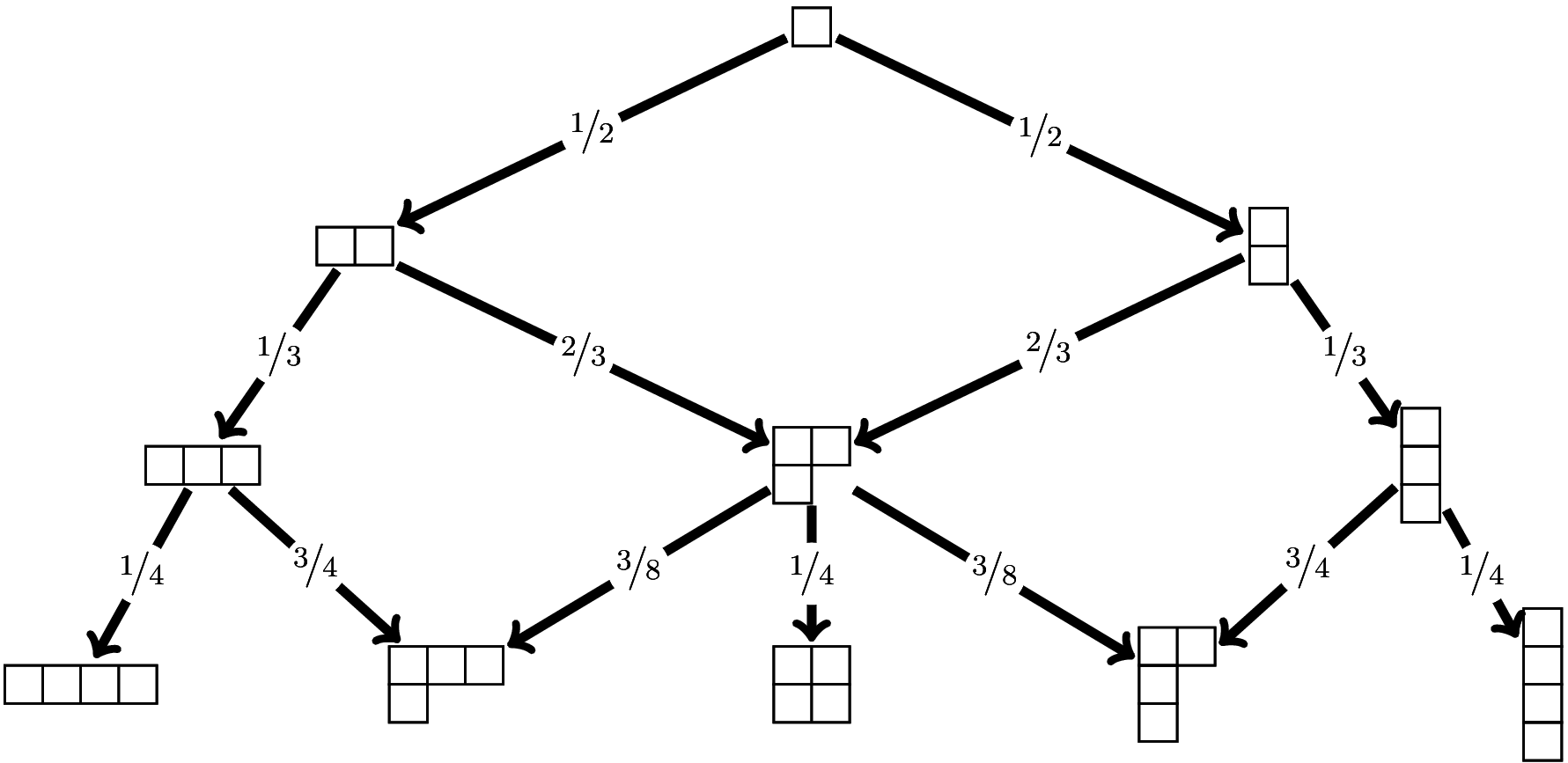

Robinson-Schensted correspondence

The RS function below returns the pair of standard Young tableaux corresponding to a given permutation by the Robinson-Schensted correspondence (it does not use the incidence matrices).

bump <- function(P, Q, e, i){
  if(length(P)==0) return(list(P=list(e), Q=list(i)))
  p <- P[[1]]
  if(e > p[length(p)]){
    P[[1]] <- c(p, e); Q[[1]] <- c(Q[[1]], i)
    return(list(P=P, Q=Q))
  }else{
    j <- which.min(p<e)
    w <- p[j]; P[[1]][j] <- e
    b <- bump(P[-1], Q[-1], w, i)
    return(list(P=c(P[1], b$P), Q=c(Q[1], b$Q)))
  }
}
RS <- function(sigma){
  out <- bump(list(), list(), sigma[1], 1)
  for(i in 2:length(sigma)){
    out <- bump(out$P, out$Q, sigma[i], i)
  }
  return(out)
}
sigma <- c(1, 3, 6, 4, 7, 5, 2)
RS(sigma)
## $P
## $P[[1]]
## [1] 1 2 4 5
## 
## $P[[2]]
## [1] 3 7
## 
## $P[[3]]
## [1] 6
## 
## 
## $Q
## $Q[[1]]
## [1] 1 2 3 5
## 
## $Q[[2]]
## [1] 4 6
## 
## $Q[[3]]
## [1] 7