
-
Drawing a Bratteli graph with R
14/08/2015
SourceHey, ergodicians! How do you draw your Bratteli graphs ? Are you using
Xfig? Are you typing rawpstricksorTikZcode? Are you crazy? I have written theBgraphR function, and it does the job without pain for you (feel free to take it here). You just have to write a R function returning the incidence matrices of the graph.Bratelli graphs - The Pascal example
A Bratteli graph, such as the Pascal graph shown below, is a graded graph whose edges only connect vertices from one level to some vertices of the next level.
Pascal graph Such a graph is defined by a sequence of incidence matrices \(M_n\). Denoting by \(c_n\) the number of vertices at level \(n\), the incidence matrix \(M_n\) is a \(c_n \times c_{n+1}\) matrix showing all connections between level \(n\) and level \(n+1\). A “\(0\)” means there’s no edge, a “\(1\)” means there’s one edge, a “\(2\)” means there’s a double edge, etc. The first three incidence matrices of the Pascal graph are
\[ M_0= \begin{pmatrix}{} 1 & 1 \\ \end{pmatrix} , \, M_1= \begin{pmatrix}{} 1 & 1 & 0 \\ 0 & 1 & 1 \\ \end{pmatrix} , \, M_2= \begin{pmatrix}{} 1 & 1 & 0 & 0 \\ 0 & 1 & 1 & 0 \\ 0 & 0 & 1 & 1 \\ \end{pmatrix} .\]
and I get them with this function:
Pascal_Mn <- function(n){
  M <- matrix(0, nrow=n+1, ncol=n+2)
  for(i in 1:(n+1)){
    M[i, ][c(i, i+1)] <- 1
  }
  return(M)
}
Given a function
fun_Mntaking a nonnegative integernas argument and returning an incidence matrix, such as thePascal_Mnfunction, myBgraphfunction, based on the diagram package, draws the corresponding Bratteli graph from the root level to a desired levelN. Its arguments are:formalArgs(Bgraph)## [1] "fun_Mn" "N" "title" "path" ## [5] "col_path" "lwd_path" "labels_path" "labels_vertex" ## [9] "USE.COLNAMES" "first_vertex" "label_root" "only_end" ## [13] "cex_vertex" "labels_edges" "cex_edge" "ellipse_vertex" ## [17] "ellipse_edge" "LaTeX" "..."The effects of most of the arguments will be illustrated below. The ellipsis
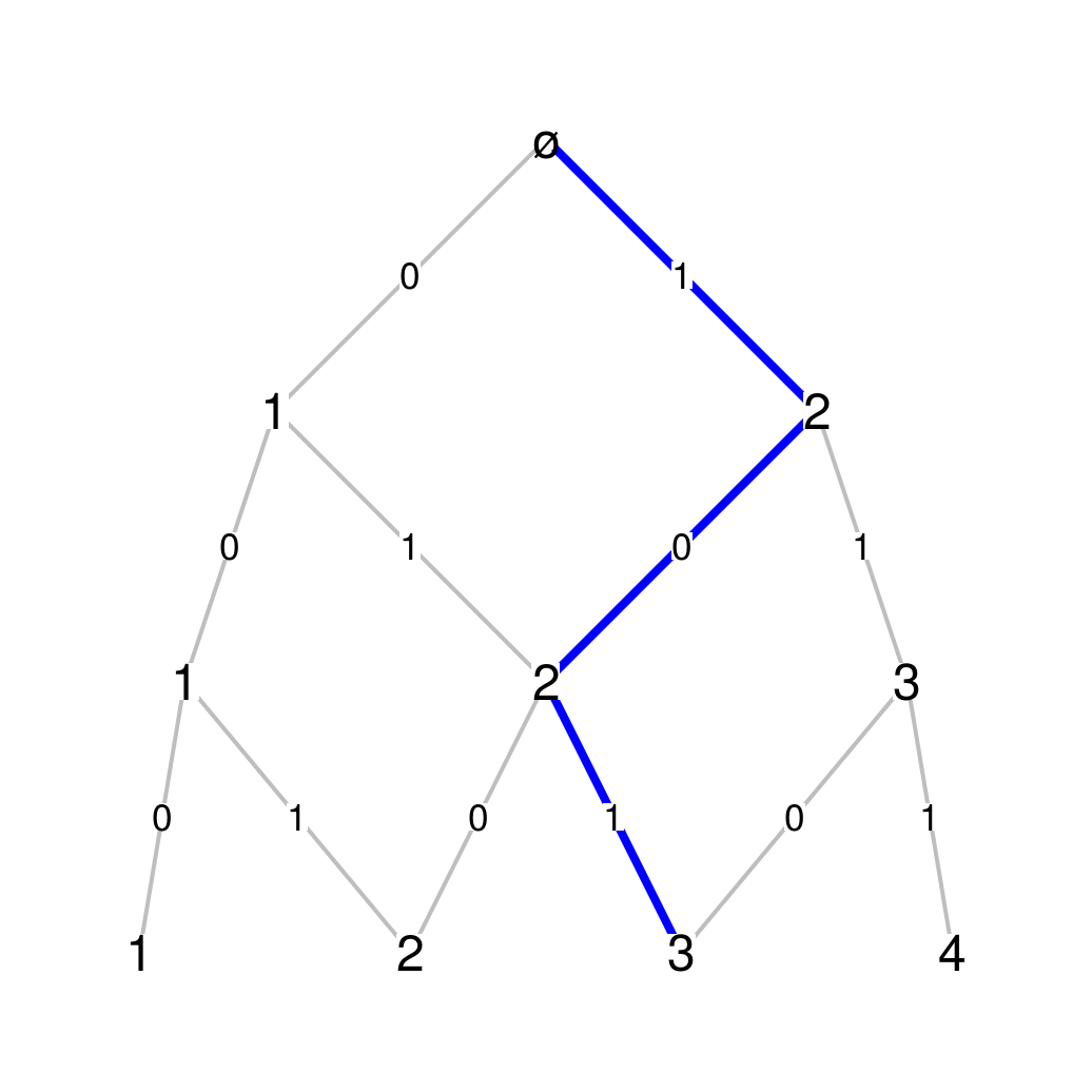
...is intended for additional arguments to the coordinates function of thediagrampackage. For example thehorargument allows to rotate the picture.The figure above has been generated by this code, except that this time we change its orientation with the
horargument:par(mar=c(.1,.1,.1,.1)) Bgraph(Pascal_Mn, N=3, path=c(1,0,1), first_vertex=1, hor=FALSE)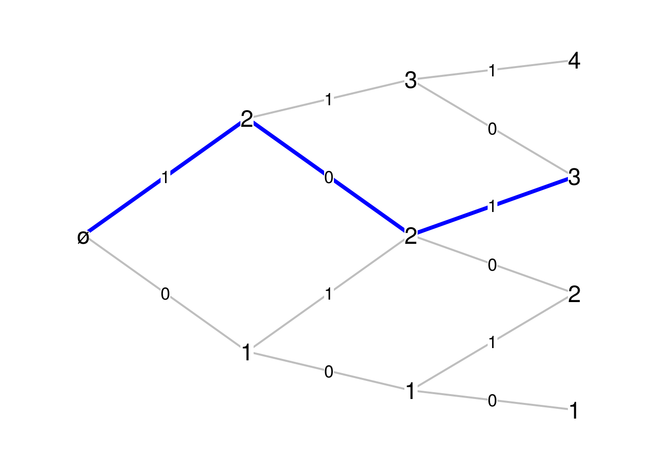
The path shown in blue on the figure, is given as the sequence of labels on the edges of this path. The
first_vertexargument, intended to be0or1, controls the label of the first vertex at each level. The user can decide to show the edge labels of the blue path only with thelabels_pathargument. By setting theonly_endargument toTRUE, only the vertex labels at the last level are shown:par(mar=c(.1,.1,.1,.1)) Bgraph(Pascal_Mn, N=3, path=c(1,0,1), first_vertex=0, labels_path=TRUE, only_end=TRUE)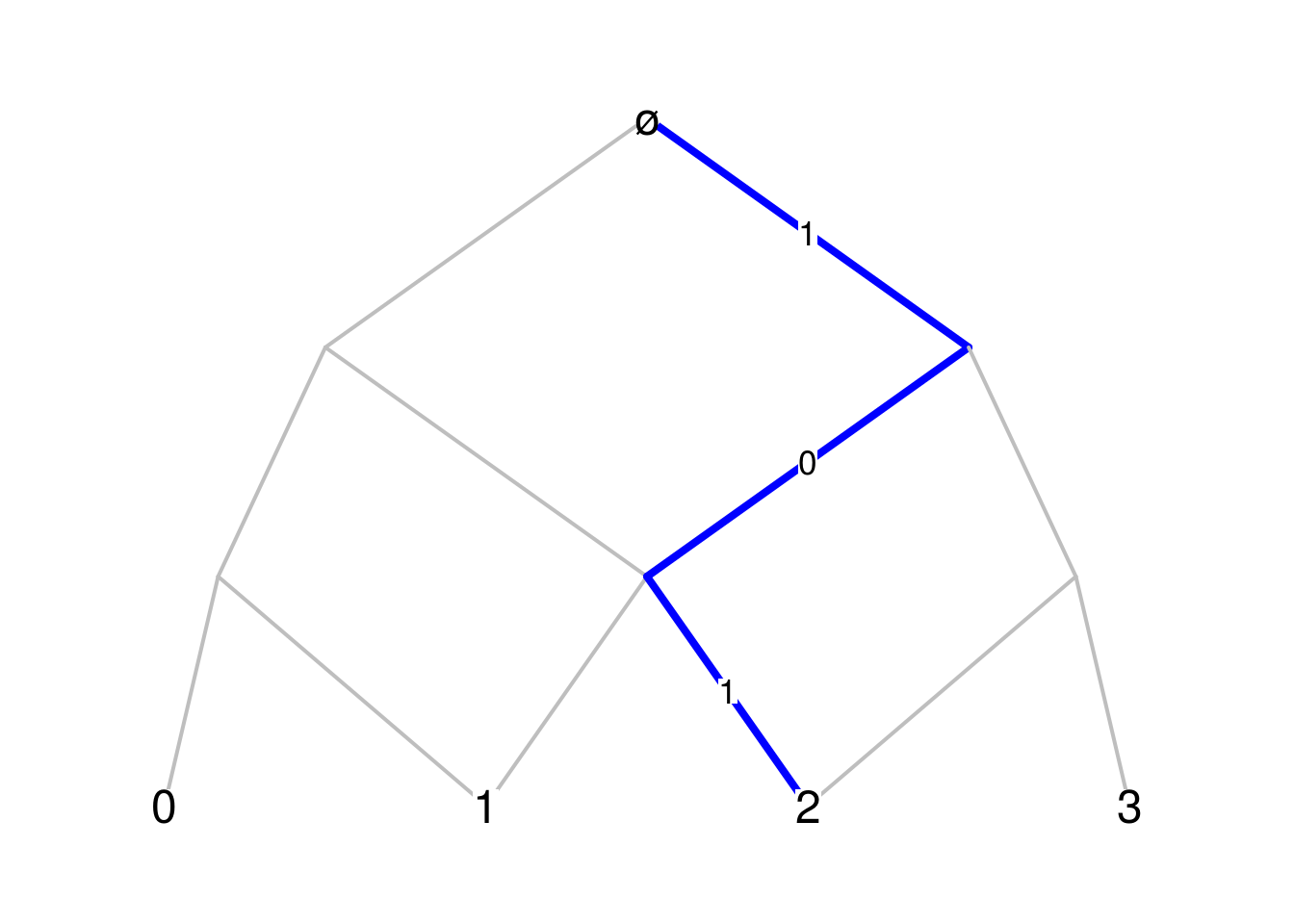
By setting the
USE.COLNAMESargument toTRUE, the vertex labels appearing at level \(n\) are the column names of \(M_n\). For example, on figure below we display the binomial numbers on the vertices Pascal graph, which give the number of paths from the root vertex. We also show the effect of theellipse_vertexargument.Pascal_Mn <- function(n){ M <- matrix(0, nrow=n+1, ncol=n+2) for(i in 1:(n+1)){ M[i, ][c(i, i+1)] <- 1 } colnames(M) <- choose(n+1, 0:(n+1)) return(M) } par(mar=c(.1,.1,.1,.1)) Bgraph(Pascal_Mn, N=4, path=c(1,0,1,1), labels_path=TRUE, USE.COLNAMES=TRUE, ellipse_vertex=TRUE)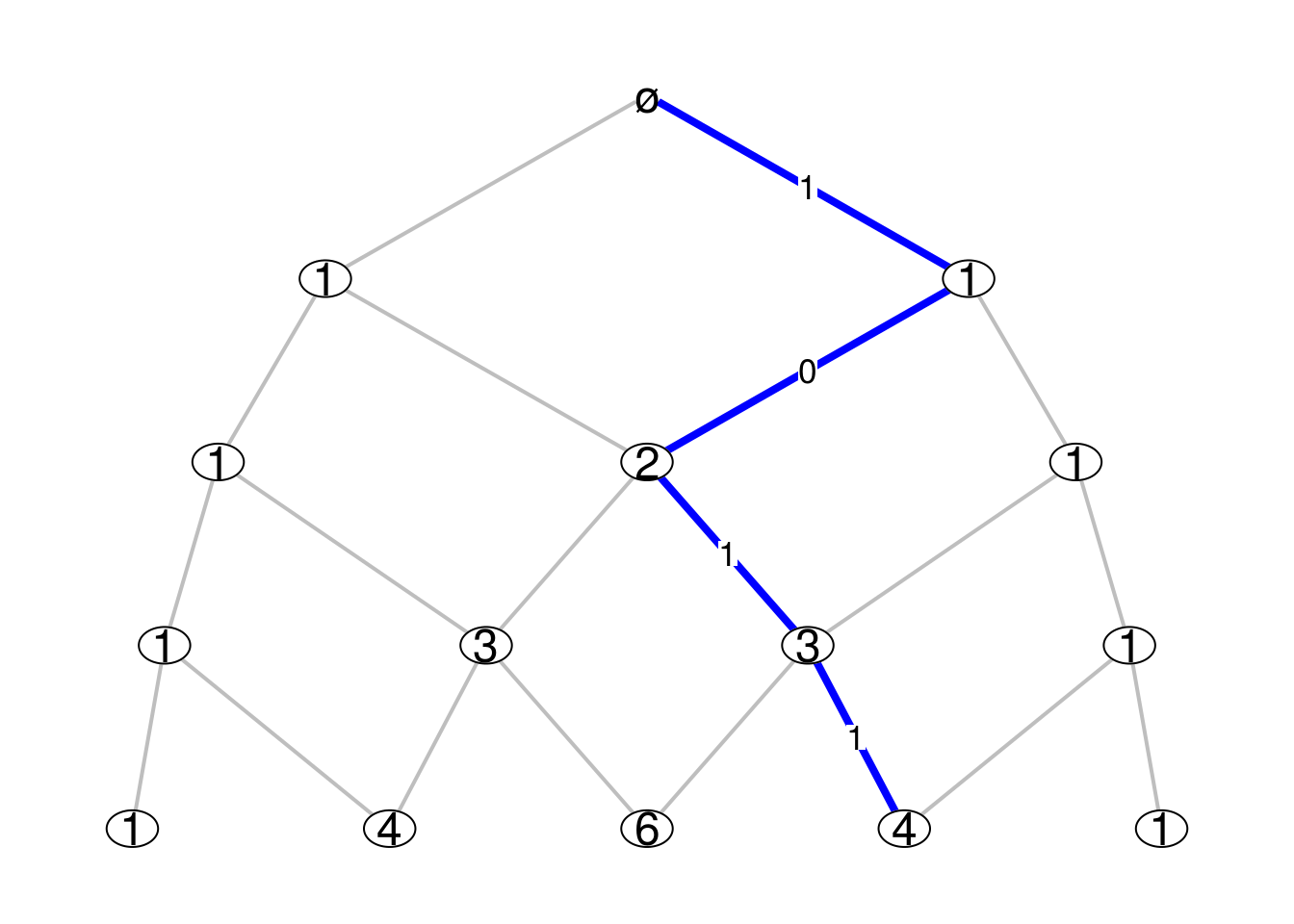
Odometers
Bratteli graphs are well-known in ergodic theory since Vershik has shown that every invertible measure-preserving transformations can be represented as a transformation on the set of paths of such a graph.
The canonical Bratteli graph of an odometer is given by incidence matrixes full of “\(1\)”:
Odometer_Mn <- function(sizes){
  sizes <- c(1,sizes)
  function(n){
    return(matrix(1, nrow=sizes[n+1], ncol=sizes[n+2]))
  }
}
par(mar=c(.1,.1,.1,.1)) fun_Mn <- Odometer_Mn(c(3,4,5)) Bgraph(fun_Mn, N=3, labels_vertex=TRUE, path=c(2,1,2), labels_path=TRUE)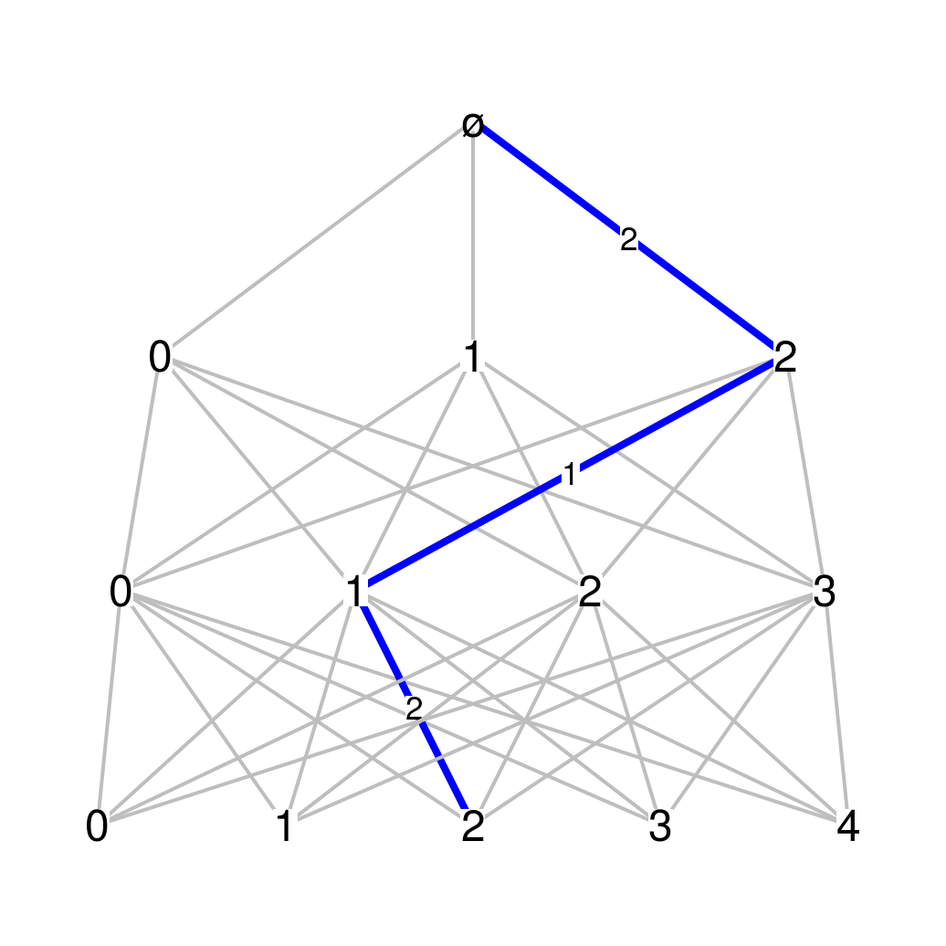
(3,4,5)-ary odometer This graph is related to Cantor expansions. For the previous example, the paths starting from the root level and going to the third level provide a representation of the Cartesian product \(\{0,1,2\}\times\{0,1,2,3\}\times\{0,1,2,3,4\}\).
Homogeneous trees
A homogeneous tree is a Bratteli graph. I use a trick to generate the incidence matrices, the same I already used before.
Tree_Mn <- function(sizes){
  function(n){
    if(n==0) return(matrix(1, ncol=sizes[1]))
    unname(t(model.matrix(~0+gl(prod(sizes[1:n]),sizes[n+1])))[,])
  }
}
As for the odometer, the paths of the tree provide a representation of a Cartesian producct, but in less compact form:
par(mar=c(.1,.1,.1,.1))
fun_Mn <- Tree_Mn(c(3,4,5))
Bgraph(fun_Mn, N=3, labels_vertex=FALSE, labels_edges=FALSE, path=c(2,1,2))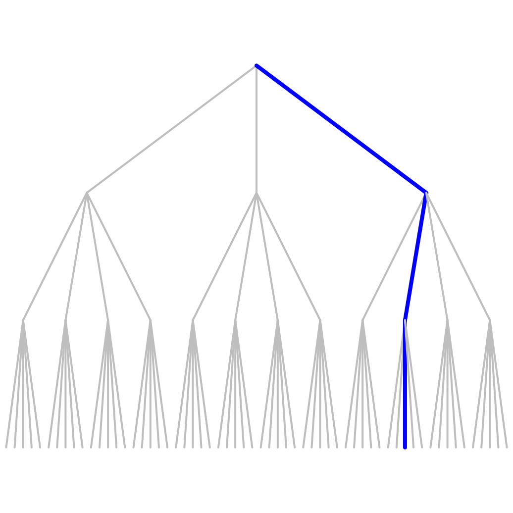
(3,4,5)-ary tree Conversion to
TikZMathematicians like \(\LaTeX\) figures. The
tikzDevicepackage allows to convert any R figure to aTikZfigure. For example we generate below the Pascal graph with the binomial numbers \({n \choose k}\) as vertex labels. We set the argumentLaTeXtoTRUEin theBgraphfunction to generate edge labels in \(\LaTeX\) math mode.Pascal_Mn <- function(n){ M <- matrix(0, nrow=n+1, ncol=n+2) for(i in 1:(n+1)){ M[i, ][c(i, i+1)] <- 1 } colnames(M) <- sprintf("${%s \\choose %s}$", n+1, 0:(n+1)) return(M) } # convert to TikZ code: library(tikzDevice) texfile <- "bratteli-Pascal.tex" tikz(texfile, standAlone=TRUE, packages=c(getOption("tikzLatexPackages"), "\\usepackage{amsmath}\n\\usepackage{amssymb}\n")) par(mar=c(.1,.1,.1,.1)) Bgraph(Pascal_Mn, N=3, path=c(1,0,1), labels_path=TRUE, USE.COLNAMES=TRUE, LaTeX=TRUE, label_root="$\\varnothing$", relsize=.6) dev.off() # convert to pdf: tools::texi2dvi(texfile, pdf=TRUE, clean=TRUE) # crop the figure (remove white margins): knitr::plot_crop("bratteli-Pascal.pdf")This is the result:
Multiples edges
My
Bgraphfunction currently handles double edges too. Let us try the Pascal graph with some double edges taken at random.Pascal2_Mn <- function(n){ M <- matrix(0, nrow=n+1, ncol=n+2) for(i in 1:(n+1)){ M[i, ][c(i, i+1)] <- sample.int(2, 1) } return(M) } set.seed(666) par(mar=c(.1,.1,.1,.1)) Bgraph(Pascal2_Mn, N=4, labels_vertex=FALSE, labels_path=TRUE, path=c(1,0,1,0))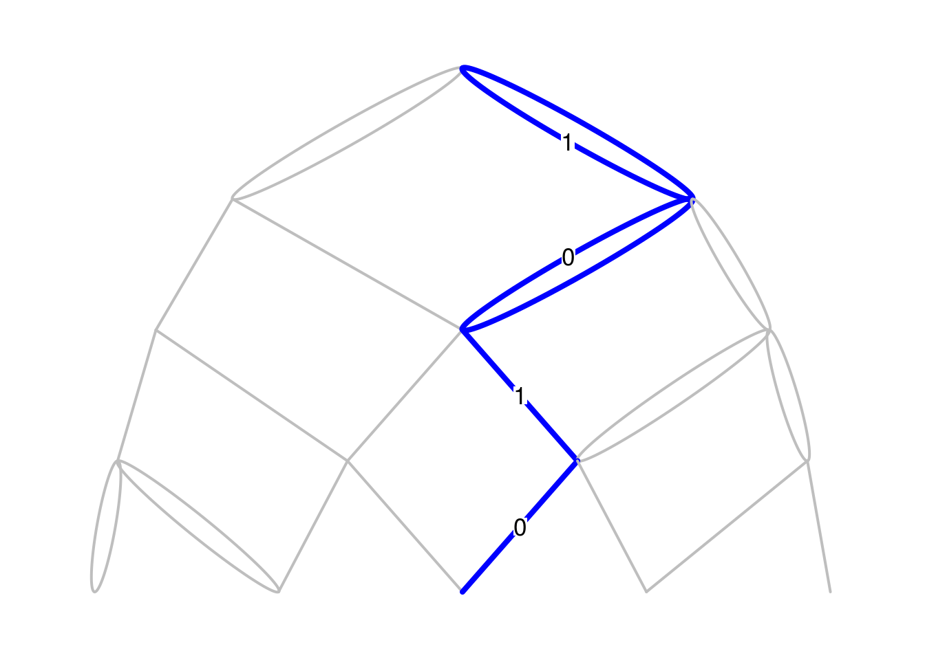
Currently, the rendering of the colored path is not correct, because the two edges of a double edge appears in color. The label edges are not correct too. This will be fixed in a next version of the
Bgraphfunction.
- Home
- About
- PoirotReproducible Blogging with R Markdown
- SlidifyReproducible html5 slides from R markdown
- R-bloggersBlog posts about R, contributed by R bloggers worldwide.
- stla.overblogMy previous blog
- Timely Portfolio A great blog about R, Javascript, and more