The tessellation package

library(tessellation)

Delaunay tessellation

The main function of the tessellation package is delaunay. It performs the Delaunay tessellation (or triangulation) of a set of points.

Let’s try it on a simple figure. We take a regular tetrahedron and we add three points at random in its interior:

tetrahedron <-
  rbind(
    c(2*sqrt(2)/3, 0, -1/3),
    c(-sqrt(2)/3, sqrt(2/3), -1/3),
    c(-sqrt(2)/3, -sqrt(2/3), -1/3),
    c(0, 0, 1)
  )
library(uniformly)
set.seed(314)
randomPoints <- runif_in_tetrahedron(
  3, tetrahedron[1, ], tetrahedron[2, ], tetrahedron[3, ], tetrahedron[4, ]
)

Let’s do a function to plot a tetrahedron. We will use it several times.

library(rgl)
plotTetrahedron <- function(tetrahedron, alpha){
  faces <- combn(4L, 3L)
  for(j in 1L:ncol(faces)){
    triangles3d(tetrahedron[faces[, j], ], color = "orange", alpha = alpha)
  }
  edges <- combn(4L, 2L)
  for(j in 1L:ncol(edges)){
    shade3d(
      cylinder3d(tetrahedron[edges[, j], ], sides = 60, radius = 0.03),
      color = "yellow"
    )
  }
  spheres3d(tetrahedron, radius = 0.05, color = "yellow")
}

Here is our tetrahedron with its three additional random points:

open3d(windowRect = c(50, 50, 562, 562))
bg3d("slategray")
plotTetrahedron(tetrahedron, alpha = 0.3)
spheres3d(randomPoints, radius = 0.04, color = "black")

Now let’s compute and plot the Delaunay tessellation of these seven points:

library(tessellation)
pts <- rbind(tetrahedron, randomPoints)
del <- delaunay(pts)
open3d(windowRect = c(50, 50, 562, 562))
material3d(lwd = 2)
plotDelaunay3D(del, color="random", luminosity = "bright", alpha=0.5)

It is not easy to visualize a 3D Delaunay tessellation. The colors are not very helpful. Something which helps a little is to plot the exterior edges as tubes. To do so, one firstly has to execute the delaunay function with the option exteriorEdges=TRUE, then one has to run the plotDelaunay3D function with the option exteriorEdgesAsTubes=TRUE:

del <- delaunay(pts, exteriorEdges = TRUE)
open3d(windowRect = c(50, 50, 562, 562))
bg3d("slategray")
material3d(lwd = 2)
plotDelaunay3D(
  del, color="random", luminosity = "bright", alpha = 0.2,
  exteriorEdgesAsTubes = TRUE, tubeRadius = 0.03, tubeColor = "navy"
)

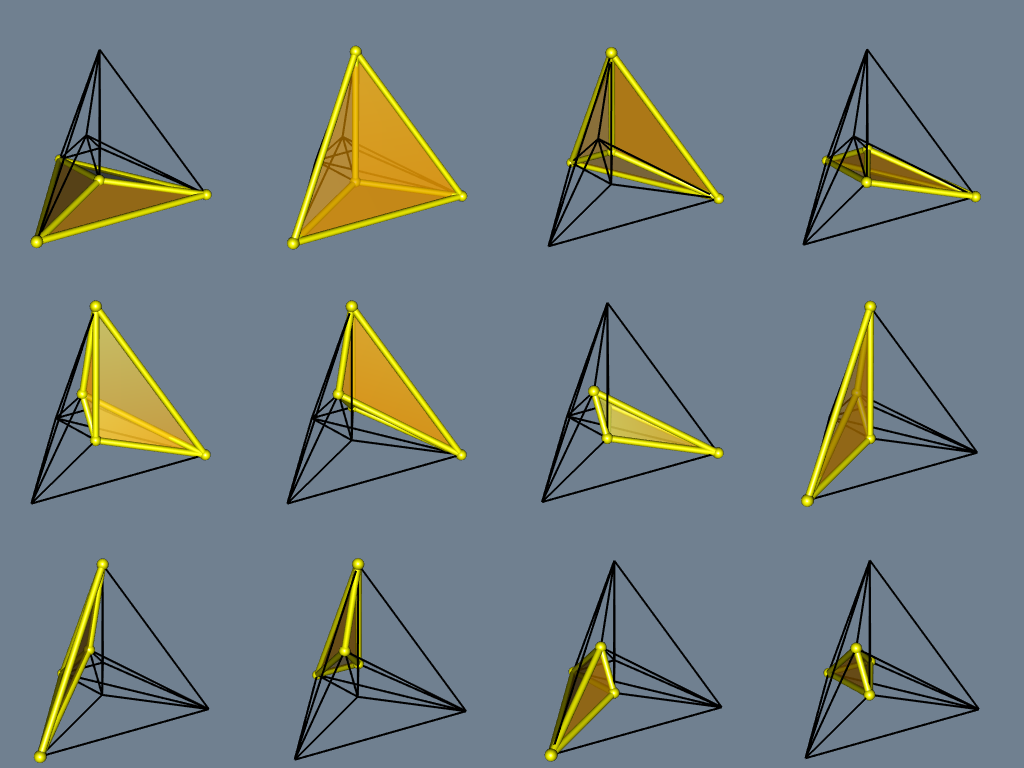
Let’s have a look at each tile, separately:

Voronoï tessellation

The Delaunay tessellation is mainly implemented in C, with the Qhull library. The Voronoï tessellation, that we will see now, is derived from the Delaunay tessellation and this derivation is implemented in R only.

The Voronoï tessellation is obtained with the voronoi function. It is restricted to its bounded cells. Let’s see what it gives on our example:

v <- voronoi(del)
#> Voronoï diagram with three bounded cells.
open3d(windowRect = c(50, 50, 562, 562))
bg3d("palegoldenrod")
material3d(lwd = 2)
plotVoronoiDiagram(v, luminosity = "dark")

Well, not very funny. Let’s add some fun. We draw two circles around the tetrahedron (two sets of points on circles, I should say):

xi_ <- seq(0, 2*pi, length.out = 91)[-1]
R <- 2
circle1 <- t(vapply(xi_, function(xi) R * c(cos(xi), sin(xi), 0), numeric(3L)))
circle2 <- t(vapply(xi_, function(xi) R * c(cos(xi), 0, sin(xi)), numeric(3L)))
circles <- rbind(circle1, circle2)
open3d(windowRect = c(50, 50, 562, 562), zoom=0.7)
bg3d("palegoldenrod")
plotTetrahedron(tetrahedron, alpha = 0.3)
spheres3d(randomPoints, radius = 0.04, color = "black")
spheres3d(circles, radius = 0.04, color = "black")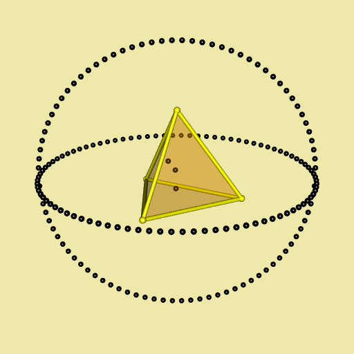

And now we gonna draw the Voronoï diagram of this object. There are seven bounded cells:

object <- rbind(tetrahedron, randomPoints, circles)
del <- delaunay(object)
v <- voronoi(del)
#> Voronoï diagram with seven bounded cells.

In fact these are the cells corresponding to the four tetrahedra vertices and the three random points.

library(viridisLite)
open3d(windowRect = c(50, 50, 562, 562))
bg3d("palegoldenrod")
plotVoronoiDiagram(v, colors = turbo(7))

Now, let’s enclose a cube with three circles, and let’s draw the corresponding Voronoï diagram:

cube <-
  rbind(
    c(-1, -1, -1),
    c( 1, -1, -1),
    c(-1,  1, -1),
    c( 1,  1, -1),
    c(-1, -1,  1),
    c( 1, -1,  1),
    c(-1,  1,  1),
    c( 1,  1,  1)
  )
xi_ <- seq(0, 2*pi, length.out = 91)[-1]
R <- 3
circle1 <- t(vapply(xi_, function(xi) R*c(cos(xi), sin(xi), 0), numeric(3L)))
circle2 <- t(vapply(xi_, function(xi) R*c(cos(xi), 0, sin(xi)), numeric(3L)))
circle3 <- t(vapply(xi_, function(xi) R*c(0, cos(xi), sin(xi)), numeric(3L)))
enclosedCube <- rbind(cube, circle1, circle2, circle3)
d <- delaunay(enclosedCube, degenerate = TRUE)
v <- voronoi(d)
#> Voronoï diagram with eight bounded cells.
library(paletteer) # provides many color palettes
open3d(windowRect = c(50, 50, 512, 512))
bg3d("palegoldenrod")
plotVoronoiDiagram(v, colors = paletteer_c("grDevices::Dark 3", 8L))

The Voronoï diagram is highly symmetric.

Option degenerate = TRUE

I encountered some cases for which I had to set the option degenerate=TRUE in the delaunay function in order to get a better Voronoï diagram. This is the case for example of this dodecahedron surrounded by three circles:

xi_ <- seq(0, 2*pi, length.out = 91)[-1]
R <- 3
circle1 <- t(vapply(xi_, function(xi) R * c(cos(xi), sin(xi), 0), numeric(3L)))
circle2 <- t(vapply(xi_, function(xi) R * c(cos(xi), 0, sin(xi)), numeric(3L)))
circle3 <- t(vapply(xi_, function(xi) R * c(0, cos(xi), sin(xi)), numeric(3L)))
circles <- rbind(circle1, circle2, circle3)
dodecahedron <- t(dodecahedron3d()$vb[-4,])
pts <- rbind(dodecahedron, circles)
del <- delaunay(pts, degenerate = TRUE)
v <- voronoi(del)
open3d(windowRect = c(50, 50, 562, 562))
bg3d("aliceblue")
plotVoronoiDiagram(v, colors = rainbow(20))

Try it with del <- delaunay(pts, degenerate = FALSE).