Plot Voronoï diagram

Plot all the bounded cells of a 2D or 3D Voronoï tessellation.

Usage

plotVoronoiDiagram(
  v,
  colors = "random",
  hue = "random",
  luminosity = "light",
  alpha = 1,
  ...
)

Arguments

v

an output of voronoi

colors

this can be "random" to use random colors for the cells (with randomColor), "distinct" to use distinct colors with the help of distinctColorPalette, or this can be NA for no colors, or a vector of colors; the length of this vector of colors must match the number of bounded cells, which is displayed when you run the voronoi function and that you can also get by typing attr(v, "nbounded")

hue, luminosity

if colors = "random", these arguments are passed to randomColor

alpha

opacity, a number between 0 and 1 (used when colors is not NA)

...

arguments passed to plotBoundedCell2D or plotBoundedCell3D

Value

No returned value.

Note

Sometimes, it is necessary to set the option degenerate=TRUE in the delaunay function in order to get a correct Voronoï diagram with the plotVoronoiDiagram function (I don't know why).

Examples

library(tessellation)
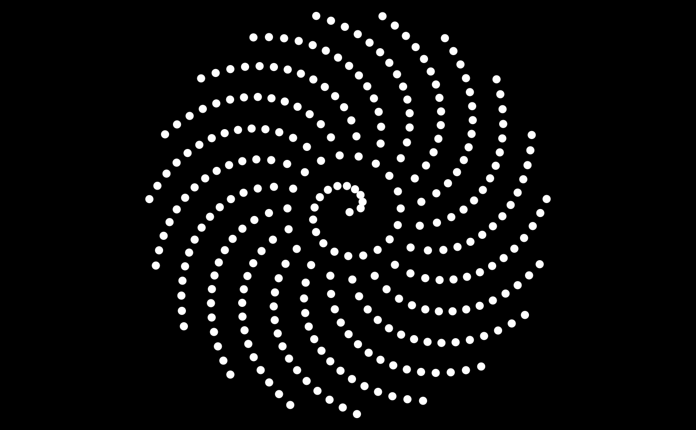
# 2D example: Fermat spiral
theta <- seq(0, 100, length.out = 300L)
x <- sqrt(theta) * cos(theta)
y <- sqrt(theta) * sin(theta)
pts <- cbind(x,y)
opar <- par(mar = c(0, 0, 0, 0), bg = "black")
# Here is a Fermat spiral:
plot(pts, asp = 1, xlab = NA, ylab = NA, axes = FALSE, pch = 19, col = "white")

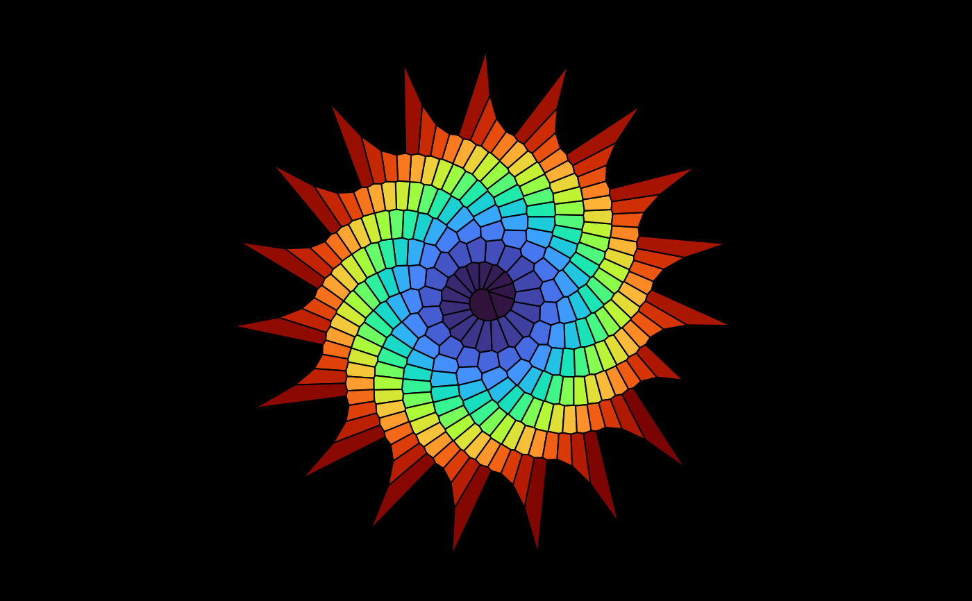
# And here is its Voronoï diagram:
plot(NULL, asp = 1, xlim = c(-15, 15), ylim = c(-15, 15),
     xlab = NA, ylab = NA, axes = FALSE)
del <- delaunay(pts)
v <- voronoi(del)
#> Voronoï diagram with 281 bounded cells.
length(Filter(isBoundedCell, v)) # 281 bounded cells
#> [1] 281
plotVoronoiDiagram(v, colors = viridisLite::turbo(281L))

par(opar)

# 3D example: tetrahedron surrounded by three circles
tetrahedron <-
  rbind(
    c(2*sqrt(2)/3, 0, -1/3),
    c(-sqrt(2)/3, sqrt(2/3), -1/3),
    c(-sqrt(2)/3, -sqrt(2/3), -1/3),
    c(0, 0, 1)
  )
angles <- seq(0, 2*pi, length.out = 91)[-1]
R <- 2.5
circle1 <- t(vapply(angles, function(a) R*c(cos(a), sin(a), 0), numeric(3L)))
circle2 <- t(vapply(angles, function(a) R*c(cos(a), 0, sin(a)), numeric(3L)))
circle3 <- t(vapply(angles, function(a) R*c(0, cos(a), sin(a)), numeric(3L)))
circles <- rbind(circle1, circle2, circle3)
pts <- rbind(tetrahedron, circles)
d <- delaunay(pts, degenerate = TRUE)
v <- voronoi(d)
#> Voronoï diagram with four bounded cells.
library(rgl)
open3d(windowRect = c(50, 50, 562, 562))
material3d(lwd = 2)
plotVoronoiDiagram(v, luminosity = "bright")